TRLINE User’s Guide
Introduction
Program TRLINE provides a laboratory for testing your solutions to homework problems in transmission line theory. This User’s Guide explains how to use TRLINE for transmission line problems commonly encountered in the introductory “Fields and Waves” course and in the “Microwave Engineering” course.
TRLINE was described in a paper published in the IEEE Transactions on Education[1].
|
|
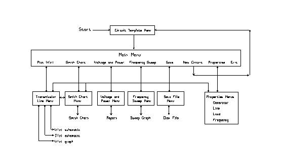
Fig. 1 The organization of the TRLINE program. |
|
Organization of the TRLINE Program
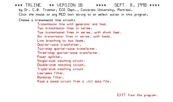
Fig. 1 shows how program TRLINE is organized. When the program is first started, the “circuit template” menu of Fig. 2 is shown. This menu asks the user to choose a circuit for study from the list shown. In all menus in TRLINE, menu choices are shown in red and are called “buttons”. Click the mouse on any red text string in any menu in the program to get an “action”. In the circuit template menu, the names of the circuits are buttons and the user clicks the mouse on a circuit name to select that circuit. Also, a saved circuit can be recalled from the disc. And in the lower right-hand corner of the screen we see an “exit button”. Most TRLINE menus have an exit button in the lower right corner. Most exit buttons return to the main menu. From the main menu the exit button quits the program.
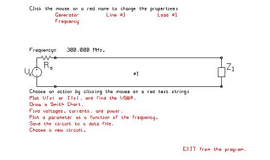
When a circuit has been chosen, the program goes to the “main menu” in Fig. 1, which gives access to a menu for each of the program’s functions. The main menu is shown in Fig. 3. The main menu is organized with a schematic diagram for the circuit across the center of the menu, “properties buttons” at the top, and action items at the bottom. The “properties buttons” are used to tell the program about the properties of each part of the circuit. Click “frequency” to specify the operating frequency. Click “generator” to specify the voltage of the generator, and its internal resistance. Click “line #1” to specify the length, characteristic impedance, and wave speed for line #1. If the circuit has, say, five transmission lines, there will be five properties buttons, one for each transmission line. Click “Load #1” to specify the resistance and reactance of the load. Note that you must type “F10” to return from each of the properties menus, as the mouse has not been implemented as yet for this style of menu! Also, the “properties buttons” appear on other menus, namely the transmission line menu and the Smith Chart menu.
The bottom of the main menu has buttons which give you access to the computations that the program can do for you. When you have set the lengths and characteristic impedances of the transmission lines, and the values of the loads, and so forth, you can save the values to a disk file by clicking “Save the circuit…”. The program asks you for a directory and file name. The program uses the extension “trl” for its data files.
The TRLINE program has four principal functions. Clicking “Plot V(z)..” gets the transmission line menu. This is used to graph the amplitude and phase of the voltage or the current on the transmission lines. There are two kinds of graphs that the program creates. The first is a schematic of the transmission line circuit with V(z) or I(z) graphed above it. The second is a graph of the voltage amplitude on any one of the lines as a function of distance, including two “markers” which let you read back values from the graph. These are described further below.
The second function is “Find voltages, currents, and power”. This gets the “voltage and power menu”. This menu lets you ask for the voltage, current and power delivered by the generator, or for the voltage, current and power delivered to any load, or for the voltage, current and power flowing into and out of any transmission line.
The third function is obtained by clicking “Draw a Smith Chart” and is used to find the input impedance of any transmission line. This obtains the “Smith Chart menu”, which can draw a Smith Chart for any transmission line in the circuit. The chart can be an impedance chart or an admittance chart. The Smith Chart display shows the Smith Chart, with the load impedance for that line being transformed back to an input impedance. The Smith Chart display reports the load and input impedance or admittance.
The fourth function of the program is obtained by clicking “Plot a parameter as a function of the frequency”. This menu lets you graph one of five parameters as a function of frequency. You can set the frequency range with a sub-menu. You can graph the input impedance as a function of frequency at any port, that is, looking into any transmission line in the circuit. You can graph the reflection coefficient or VSWR looking into any transmission line. You can plot the return loss. And you can graph the transmission loss between any two junctions in the circuit. These are usually chosen as the input terminals and the load terminals. The frequency-sweep graphs include two markers that can read back points from the graph. Also, there is a “snap” function which lets you snap the position of the markers to a desired level, say –20 dB return loss. Then the program reports the bandwidth between the markers.
The following describes each of the program’s functions in more detail, with some examples.
|
|
Fig. 2 The “circuit template” menu. |
|
|
|
Fig. 3 TRLINE’s main menu. |
|
Choosing a Circuit
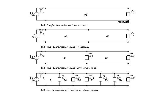
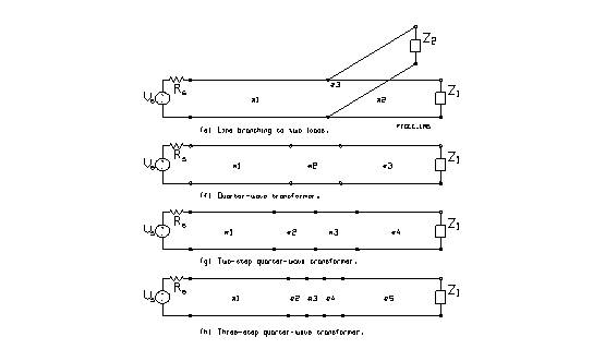
The “circuit template” menu of Fig. 2 offers a variety of circuits that are useful in learning about transmission lines at the elementary and intermediate level. The simple circuit of Fig. 4(a) consists of a generator, one transmission line, and a load. It is used, as discussed below, to demonstrate travelling waves and standing waves, and explore mismatch. It is also used to show the operation of the Smith Chart. Two transmission lines in series, Fig. 4(b) is used to show transmission from a line of say 50 ohm to a line of a different characteristic impedance, say 25 ohms or 100 ohms. Fig. 4(c) puts a shunt load at the junction and provides an exercise in the use of the Smith Chart to find the input impedance. Also the length and characteristic impedance of the interconnecting line can be chosen to try to obtain a specified relationship of the voltage amplitude and phase across the two loads.
|
|
Fig. 4 Circuit templates offered by program TRLINE. |
|
Fig. 4(d) provides a circuit template with six transmission lines in series, including a shunt load across each junction. This circuit can be used to model a variety of problems. By setting the loads to high values, we open-circuit them. Then the circuit can model a multi-step impedance matching transformer, though explicit circuit templates have been provided for one-, two-, and three-step transformers. The circuit can model a waveguide-fed slot array, where the line lengths are chosen to phase the voltage across the loads in a specified way.
|
|
Fig. 4 continued |
|
Fig. 4(e) is a problem commonly given as homework, consisting of a transmission line that branches to two loads of different, complex-valued characteristic impedance. The student must find the input impedance, then the power delivered to each load impedance. The problem of choosing the line lengths and characteristic impedances to better match the source can be considered.
Fig. 4(f), (g) and (h) provide circuit templates for one, two and three-step quarter-wave transformers. The default values for the line lengths, characteristic impedances and the frequency achieve a good match in these circuits. This is convenient for classroom demonstration of the program, for the circuits can be invoked rapidly from the circuit template menu. The match can be demonstrated by graphing the amplitude of V(z) on each transmission line, and the frequency sweep feature used to demonstrate the bandwidth of each transformer.
|
|
Fig. 4 continued |
|
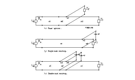
Fig. 4(i) is a circuit for a power splitter. A transmission line branches to two lines of equal characteristic impedance, terminated with matched loads. A quarter-wave transformer is included to match the source to the branch. We can note in passing that the TRLINE program could solve this circuit with two- or three-step transformers, but the program does not provide a circuit template. The user could construct a “trl” data file to create such a circuit.
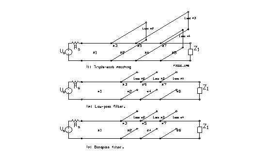
Fig. 4(j), (k) and (l) provide circuit templates for single, double, and triple stub matching. These circuits have default values that achieve a good match, again for classroom demonstration purposes.
|
|
Fig. 4 continued |
|
Fig. 4(k) and (l) use open-circuited stubs to demonstrate a low-pass and a bandstop filter, respectively. These circuit templates are actually the same as the triple stub matching circuit, with the loads on the stubs set to high impedances rather than short circuits. The low-pass filter comes with default values that can be used in classroom demonstration to show the voltages on the lines and the transmission loss. Similarly, the bandstop filter is set with values useful for demonstrating the idea.
The following describes the features of the program that can be used to demonstrate the operation of these various circuits.
Setting the Component Values: Properties Menus
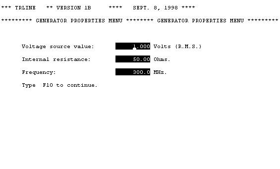
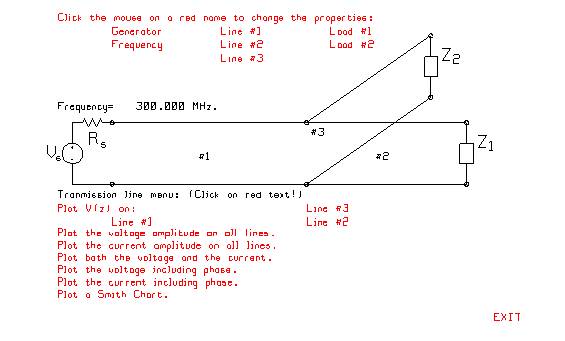
Start the TRLINE program and choose a circuit, say the transmission line branching to two loads. This gets the main menu, shown in Fig. 5. To set the component values to correspond to those of the circuit we wish to solve, we use the “properties buttons” across the top of the screen. Recall that “buttons” in the program are red text strings, so you can click the mouse on any red text string to get a function in the program. Click on “Generator” to get the generator menu of Fig. 6. This menu has fields to specify the R.M.S. value of the open-circuit voltage of the generator, and the generator’s internal resistance. Also, the frequency can be set. You must use the arrow keys to navigate from one field to the other in this style of menu. Also, the “enter” key moves the cursor from one field to another, as well as the “tab” key. Type function key “F10” to return to the main menu, or click the mouse on the “Type F10…” line.
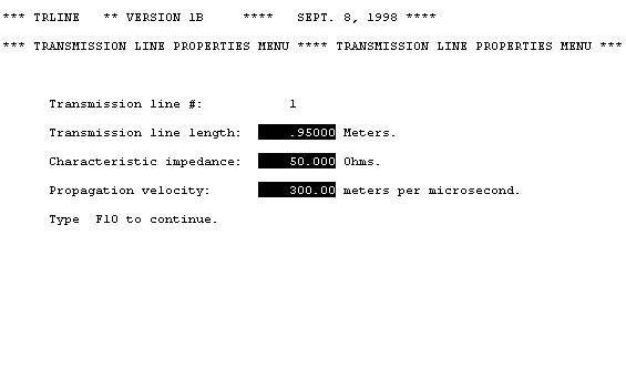
To set the properties of the transmission line in Fig. 5, click the mouse on “Line #1” at the top of the screen to get the transmission line properties menu of Fig. 7. This menu has fields for typing the characteristic impedance of the line, the length of the line and the phase velocity of waves on the line. Type F10 to get back to the main menu.
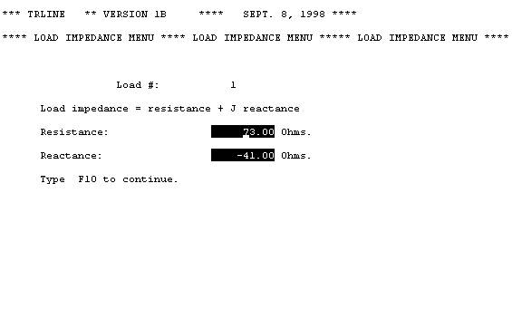
Fig. 8 shows the properties menu for a load. Type the resistance and the reactance into the fields. Version 1B of TRLINE offers only constant-impedance loads. Future versions may offer parallel RLC loads, having an impedance that varies with frequency.
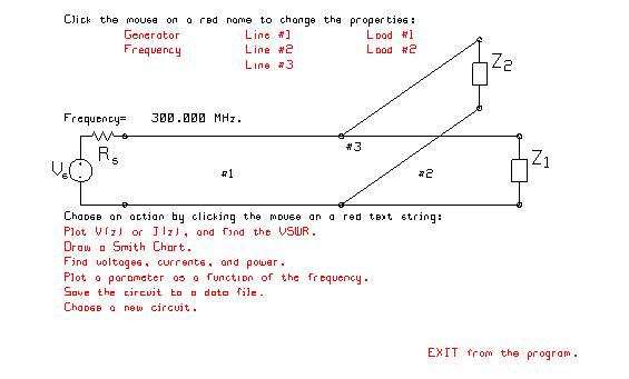
Fig. 5 The main menu showing the “properties buttons” across the top of the screen.
|
|
Fig. 6 The properties menu for the generator. |
|
|
|
Fig. 7 The properties menu for a transmission line. |
|
|
|
Fig. 8 The properties menu for a load. |
|
Graphing the Voltage on the Transmission Lines
The “transmission line menu” in the organization chart of Fig. 1 is used to graph the magnitude and phase of the voltage and current on the transmission lines making up the circuit. To find the transmission line menu, start the program, and choose a circuit, say the line that branches to two different loads to get the main menu of Fig. 5. Click the mouse on “transmission line menu”, which gets the menu of Fig. 9. This menu lets the user graph voltage and current as a function of position on any of the transmission lines. Across the top of the menu we find the “properties buttons” used to changes the parameters of the generator, lines and loads, as discussed above. At the bottom we find the menu’s action buttons.
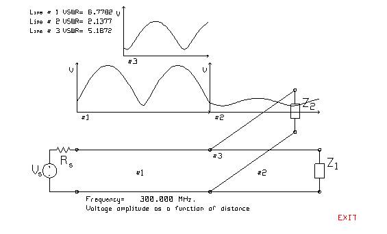
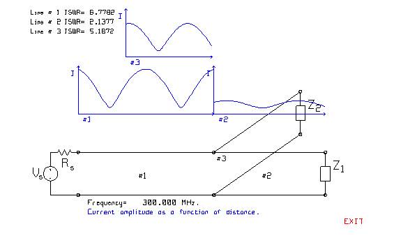
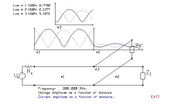
Click “Plot the voltage amplitude…” to get the graph of Fig. 10 showing the amplitude of the voltage as a function of position on all three transmission lines. The branching line’s voltage is shown across the top of the screen. In the menu of Fig. 9, click “Plot the current” to get the current standing-wave pattern of Fig. 11. Both current and voltage can be seen by clicking “Plot both the voltage and the current” to get the drawing of Fig. 12. We see that where the voltage has a standing-wave maximum, the current has a standing-wave minimum.
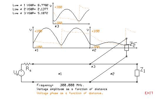
We can add phase to the standing-wave pattern. Thus click “Plot the voltage including phase” and we get the graph of Fig. 13. On line #1 the standing-wave ratio is large, and the phase is almost constant with distance, and has abrupt reversals at the minima in the standing wave pattern. Line #1 has a better match, and the phase more clearly shows the progressive-phase-with-distance expected of a travelling wave.
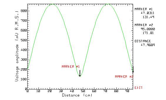
To obtain a labeled graph of voltage as a function of position on any one of the transmission lines, click the line name (in red) in the menu of Fig. 9. Thus to graph the voltage on line #1, below “Plot V(z)”, click “Line #1”. This gets the graph of Fig. 14. We see a labeled voltage axis and a labeled distance axis. The graph shows a standing-wave pattern. The display includes two “markers” for reading back values. Click the mouse on the red string “Marker #1”, then click the mouse again on the desired position of the marker. The marker jumps to the new location and the distance and voltage are reported in the upper right hand corner of the screen. The distance between the markers is also reported, hence the markers are easily used to determine the distance from the load of the first standing-wave maximum and of the first minimum.
|
|
Fig. 9 The “transmission line” menu. |
|
|
|
Fig. 10 The voltage amplitude as a function of position on the three transmission lines. |
|
|
|
Fig. 11 The current amplitude as a function of position on the three transmission lines. |
|
|
|
Fig. 12 Both the voltage and the current as functions of position on the three transmission lines. |
|
|
|
Fig. 13 The amplitude and the phase of the voltage as a function of position on the three transmission lines. |
|
|
|
Fig. 14 The voltage amplitude on a labelled graph, including markers to read out values. |
|
Smith Chart and Input Impedance
The last button on the transmission line menu in Fig. 9 is “Plot a Smith Chart”. The main menu in Fig. 5 has a “Draw a Smith Chart” button. Both these buttons get the Smith Chart Menu of Fig. 15. This menu has the properties buttons across the top so that we can easily change the line lengths and so forth. The bottom of the menu has a button labeled “Switch to an Admittance Chart” which is used to toggle the program between computing impedance and computing admittance. Across the center, below the circuit schematic, there is a button for each transmission line. If we click the mouse on the button for, say, Line #2, we obtain the Smith Chart calculation the input impedance shown in Fig. 16.
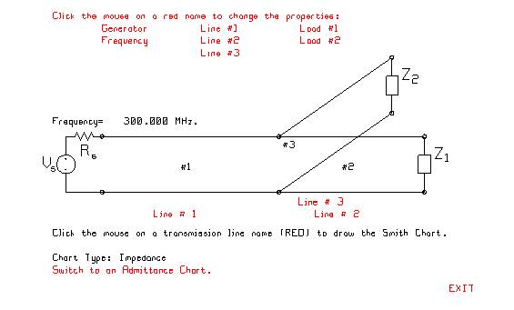
Fig. 15 The Smith Chart Menu is used to draw Smith Charts and calculate input impedance.
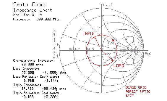
Fig. 16 The Smith Chart for Line #2 in the circuit of Fig. 15.
The “DENSE GRID” button at the lower right is used to increase the number of circles used for the Smith Chart axes; the sparse grid shown in the figure is effective on the computer screen. The “ASPECT RATIO” button lets the user adjust the ratio of vertical units to horizontal units used to draw the graphics so that the Smith Chart circle will be round. This is dependent on the vertical sweep adjustment of the monitor, too. The red circle on the Smith Chart illustrates the circle that would be drawn on a paper copy of the Smith Chart to transform the load impedance on Line #2 into its input impedance. The text at the lower left reports the load impedance and reflection coefficient, and the input impedance and reflection coefficient. The “EXIT” button returns to the Smith Chart menu.
The Power Menu
In the main menu of Fig. 5, click the button labeled “Find voltages, currents and power.” This gets the power menu of Fig. 17. This menu lists one button for each part of the circuit across the bottom of the screen. Click “Generator” to get the power delivered by the generator as in Fig. 18. This screen reports the voltage and current at the generator terminals, the input impedance into the transmission line circuit, and the power delivered by the generator to the circuit.
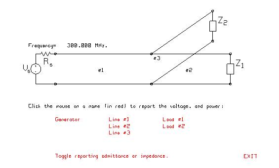
Fig. 17 The power menu.
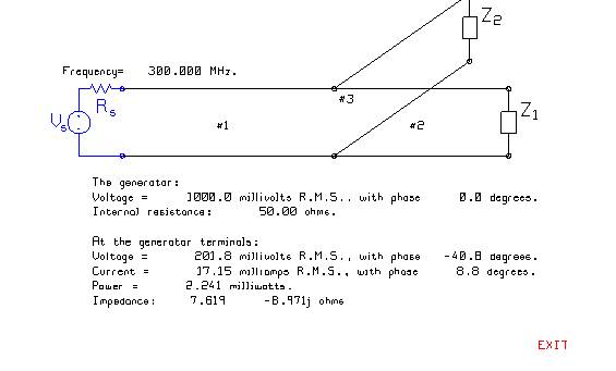
Fig. 18 The power delivered by the generator.
Click “Line #1” in the power menu of Fig. 17 to get the power flow on transmssion line #1 of the circuit, shown in Fig. 19. This screen reports the voltage, current and impedance at the input to this transmission line, and the power flowing into the line. Also we see the voltage and current at the output of the line, and the input impedance into the next section of the transmission line circuit. The power flow out of this section of the line is given. Since TRLINE solves lossless transmission line circuits, the power flow into any line must equal the power flow out.
Fig. 20 shows the report for load #1. We see the voltage and current at load #1, and the power delivered to the load. Using the power flow menu we can determine how much power the source delivers, and how much of that power finds its way to each of the loads.
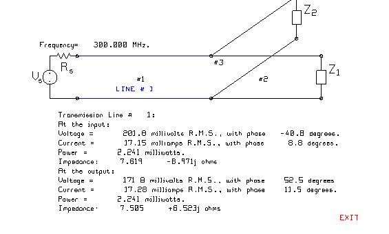
Fig. 19 The power flow report for transmission line #1.
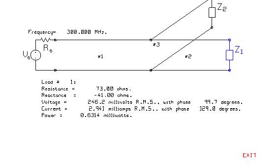
Fig. 20 The voltage, current and power at load #1.
Frequency Response
It requires extensive calculation to determine the behavior of a transmission line as a function of frequency. The TRLINE program provides a menu for plotting various parameters over a specified frequency range. Load the “double stub matching” circuit template from the entry menu of Fig. 2 as an example of a circuit for which the frequency response is of interest. The matching circuit is designed to provide a match at 300 MHz; plot the voltage on the transmission lines at 300 MHz and verify that there is a good match at the input. How wide is the bandwidth of the match.
Click “Plot a parameter as a function of frequency” in the main menu of Fig. 5 to get the frequency response menu of Fig. 21. The program can plot five parameters as a function of frequency: input inpedance, VSWR, reflection coefficient, return loss and transmission loss.
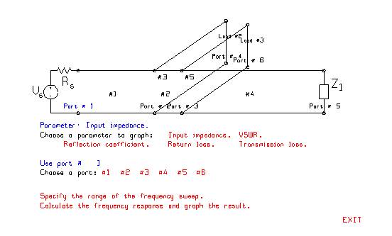
Fig. 21 The frequency response menu.
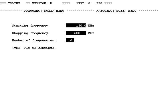
Fig. 22 The frequency range menu.
Click “input impedance” and then click one of the “ports” listed after “Choose a port”. Then click “Specify the range of the frequency sweep” to get the menu of Fig. 22, which asks for a starting frequency for the sweep, an ending frequency and a frequency step. We will choose a sweep from half the nominal frequency of 300 MHz to twice that frequency. Click F10 to return to the sweep menu and then click “Calculate the frequency response…” to get the input resistance and reactance as a function of frequency as in Fig. 23. For this circuit the input impedance is rather complicated as a function of frequency. Although the input impedance is 50 ohms with zero reactance at the “design” frequency of 300 MHz, it rapidly rises to more than 100 ohms and it is clear that the “match” is rather narrow in bandwidth. At some frequencies the line lengths to the loads transform the loads into high impedances at the input.
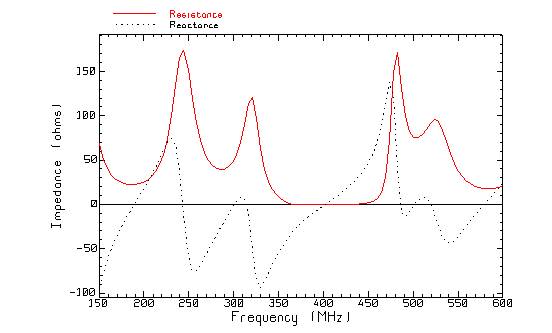
Fig. 23 The input impedance as a function of frequency.
Clicking “VSWR” on the menu of Fig. 21 then clicking “Plot…” gets the voltage standing wave ratio at the specified port, as a function of frequency as in Fig. 24. The VSWR is close to unity at the design frequency of 300 MHz but rises rapidly with increasing frequency. This menu provides two “markers” that can be moved with the mouse to read back points on the curve. Thus we can determine that at 299.9 MHz the VSWR is 1.10; but at 321.4 MHz the VSWR is 3.01. By choosing a narrower frequency range we can determine the minimum VSWR more accurately. Thus if I choose 285 MHz to 315 MHz, I can use one of the markers to determine that the best match is at 300.4 MHz with a VSWR of 1.01. To find the bandwidth for a VSWR of less than 1.1, click “SNAP MENU” and specify 1.1 as the target value. This obtains Fig. 25. The bandwidth is 298.4 to 302.3 MHz.
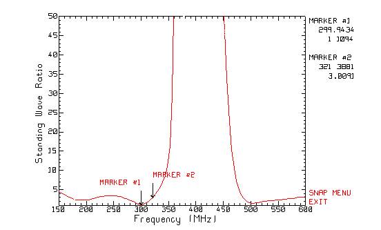
Fig. 24 The VSWR as a function of frequency.
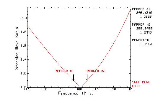
Fig.
25 The VSWR from 285 to 315 MHz, with the markers set to show the bandwidth for
a VSWR of less than 1.1.
Choosing “reflection coefficient” in the frequency response menu of Fig. 21 then clicking “Calculate…” gets the reflection coefficient magnitude as a function of frequency as in Fig. 26. Here the markers have been “snapped” to show the bandwidth for a reflection coefficient of less than 0.2.
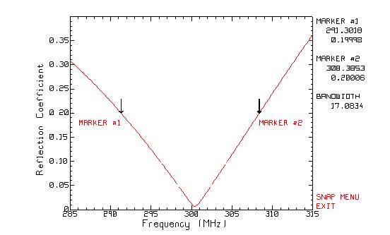
Fig. 26 The reflection coefficient as a function of frequency.
It is more common to graph the “return loss” as a function of frequency. The “return loss” is the reflection coefficient expressed in dB. Click “return loss” in Fig. 21 then “Calculate..”. Use the snap function to set the markers to –20 dB to get the return loss as a function of frequency in Fig. 27. The bandwidth for a return loss better than 20 dB is from 296.1 to 304.4 MHz.
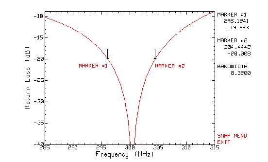
Fig. 27 The return loss as a function of frequency, with the markers set to show the bandwidth for a return loss better than 20 dB.
Finally, “transmission loss” is the ratio of the output voltage to the input voltage, expressed in dB. Click “transmission loss” in the menu of Fig. 21, and select the input port or “from” port as #1 and the output port or “to” port as #5. Then click “Calculate…” to get the graph in Fig. 28. Marker #1 has been set to show that the transmission loss is only 0.0005 dB at the nominal frequency of 300 MHz. Marker #2 shows that at 304.4 MHz, where the return loss is 20 dB, the transmission loss is 0.04 dB.
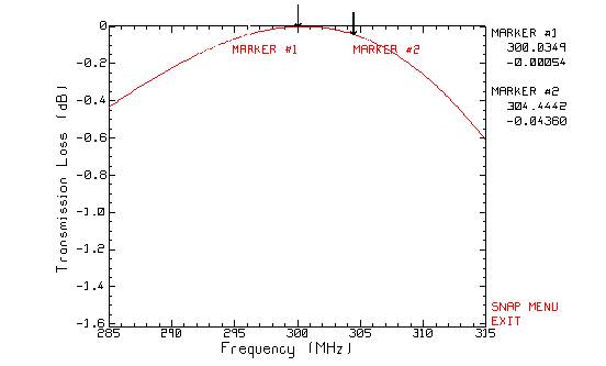
Fig. 28 The transmission loss as a function of frequency.
Saving the Circuit to a File
The main menu of Fig. 5 has a button labelled “Save the circuit to a file” which is used to create a data file with extension “bnc” containing all the information about a circuit. If you have entered your generator voltage and impedance, your line lengths, impedances and wave speeds, and your load values, you may wish to continue working on the circuit later without reentering all these values. Use the “save” function to create a “bounce” data file. The program asks you for a directory name and a file name. Then when you restart the program, click “Read a saved circuit…” in the entry menu of Fig. 2 and recall your circuit from the saved file. The program remembers the name of the last circuit you saved, which is handy to quickly recalling your previous work.
Conclusion
Program TRLINE’s circuit templates make it easy for the student to study typical circuits encountered in a “fields and waves” course or in a “microwave circuits” course. TRLINE illustrates the basic behavior of transmission lines well. TRLINE provides a computational “laboratory” for students to test their solutions to pencil-and-paper homework problems involving series transmission lines, transformer matching, stub matching, and branching circuits. TRLINE’s frequency sweeping capabilities make it possible to study the bandwidth of these circuits. TRLINE provides circuit templates for more advanced topics such as power splitters, bandpass and bandstop filters.
Reference
C.W. Trueman
March 4, 1997.
Revised Sept. 24, 1998.